GeoGuessrBot: Predicting the Location of Any Street View Image
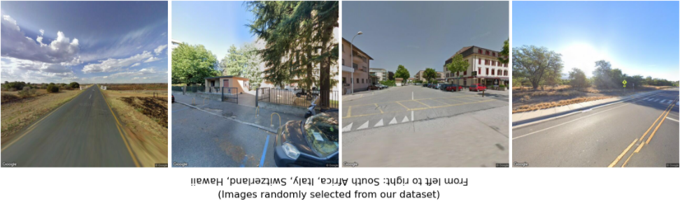
Which countries are the images below from? Take a moment to think about it. When you are ready, compare your guesses to the solutions (the upside-down caption beneath the images).
Predicting the location of Street View images is a fun and difficult task. Online games such as GeoGuessr challenge players to do just this. Players scour for clues in the landscape, signage, inhabitants, road markings, and the position of the sun in the sky. To date, no one has built a model to solve this task. A model that can accurately predict the location of a Street View image would also have useful applications. It could help law enforcement determine the location of photos. It could add metadata to images, creating extra features that could be helpful for solving other tasks.
Our contributions are as follows:
- A novel dataset consisting of 97,068 Street View images uniformly sampled from 87 countries
- A model that predicts an image’s country with 75% accuracy (94% top-5 accuracy)
- A model that predicts the US State of an image with 64% accuracy (90% top-5 accuracy)
- A model that correctly predicts an image’s location within 25km (16 miles) in 9% of cases, within 200km (124 miles) in 39% of cases, or within 750km (466 miles) in 72% of cases
For a live demo of all three models, visit GeoGuessrBot.com. The data and our code is avaiable at github.com/vdefont/geoguessr.
Table of Contents
- The Dataset
- Country Prediction
- US State Prediction
- Location Prediction
- Countries That Resemble US States
- Appendix
- Footnotes
The Dataset
There previously existed no dataset of Street View images uniformly sampled from around the world. There do exist large-scale worldwide image datasets, as in Im2GPS 1, PlaNet 2, and Müller-Budack et al 3. Yet these datasets, while quite large (with respective sizes of 6m, 100m, and 126m), are all comprised of images from Flickr and other photo-sharing sites. This makes them unsuitable for our task for two reasons: first, most of the dataset is not street view images, and second, the dataset is biased towards places where people take many pictures, such as tourist attractions and big cities. We would instead like a dataset that is more uniformly distributed across the globe, including not just famous cities but also more obscure or mundane locations.
There do exist two datasets solely consisting of Street View images, yet with more narrow scope. Zamir and Shah 4 scrape 100,000 Street View images from Pittsburgh, PA and Orlando, FL. Suresh et al 5 scrape 600,000 Street View images from across the United States. Although this latter dataset is also not quite broad enough in scope, we will still use it in this work to improve our geolocation accuracy for images taken in the US.
The team at GeoGuessr provided us with a list of 100,000 locations uniformly distributed around the world (see the appendix for an analysis of how uniform the distribution is). We removed duplicate images and invalid locations, and discarded data from countries with fewer than fifty examples. This left us with 97,068 unique locations. For each location, we scraped an image from Google’s Street View API, choosing a random direction to look (ranging between north, south, east, and west).
We split our dataset into training, validation, and test sets of size 77,654, 9,707, and 9,707 respectively (roughly an 80% / 10% / 10% split).
Country Prediction
We fine-tune a pre-trained resnet101, using a head with one hidden layer. We apply lots of data augmentation during training (but not at test time). Our results are as follows:
| Top-1 | Top-3 | Top-5 | |
|---|---|---|---|
| Our Model | 75.3% | 89.9% | 93.7% |
| Naive Model | 19.3% | 31.2% | 41.8% |
The naive model always predicts the countries that appear most often in the training set (in order, these are the US, France, Russia, Japan, and the UK). The accuracy per country is as follows:
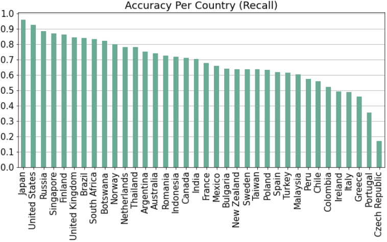
This figure shows accuracy computed across both the validation and test sets (our accuracy was very similar for both as we did not tune extensively). We only include countries with at least 100 images across the validation and test set, as the accuracy would be subject to too much variance for countries with very few images. The accuracy is quite high for most countries, but is low for a few of them. Let’s plot a confusion matrix to find out why:
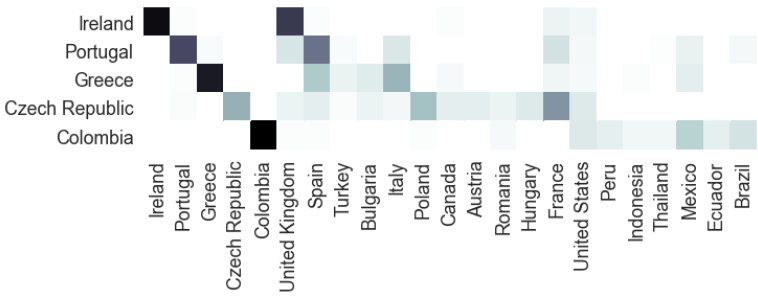
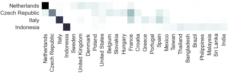
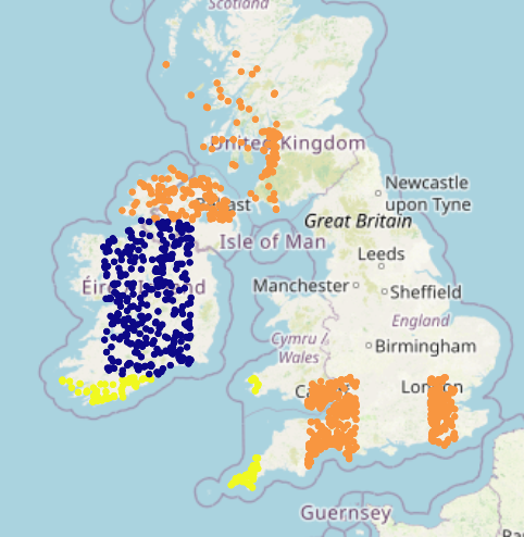
Each row shows all images from a given country, and the columns show the countries our model predicted for those images. It makes sense that images from Ireland are often misclassified as being in the UK. The two countries look quite similar, so the model errs on the side of predicting the UK since our dataset contains more images from the UK than from Ireland. The other four countries shown also follow this pattern, getting confused for countries that look similar to them, and which are often more populous and thus better-represented in our dataset.
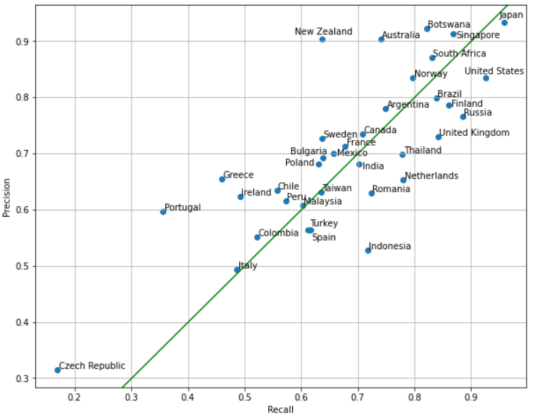
So far, we have only considered recall, but precision is also a useful measure of accuracy. Let’s examine the precision and recall for each country:
In this context, we find it useful to think of precision and recall as follows:
- Country X has low recall: “Many locations in Country X resemble a different country”
- Country Y has low precision: “Many locations in other countries resemble Country Y”
Observe that some countries have a lower precision than recall, such as the Netherlands and Indonesia. Let’s plot a confusion matrix for those countries, along with a couple other countries that have a low recall in absolute terms. Note that each row contains all images predicted to be in Country X, and each column shows where those images actually were.
US State Prediction
We use the dataset from Suresh et al 5, which contains 600,000 images annotated by state. The authors created this dataset by collecting 150,000 unique locations evenly distributed across all 50 states (so each state has 3,000 locations). For each location, they scraped four images: one looking in each cardinal direction (north, east, south, and west). The authors split the data into 500,000 training images and 100,000 test images. They built a model that took a set of four images as input, and predicted the state.
To build our model, we fine-tune a pre-trained resnet101 as we did for our country model. We experimentally found that our accuracy was higher when we built a model that takes one image as input, and made predictions by averaging the model’s output over the four images corresponding to each location (as opposed to building a model that takes all four images as input as the authors did). For a fair comparison, we use the same train / test split as the authors. We further split the training set into 450,000 training images and 50,000 validation images. Here are the results:
| Top-1 | Top-3 | Top-5 | |
|---|---|---|---|
| Suresh et al 5 | 34.8% | 59.5% | 71.1% |
| Ours | 92.4% | 98.0% | 99.3% |
| Ours (individual images) | 64.1% | 83.8% | 90.3% |
Note that we also report the results of our model when applied to individual images (as opposed to averaging over the four images for each location), as this corresponds to how we will use the model in the rest of this work. From this point forward, all reported accuracy statistics will be computed using the individual-image method. We examine the accuracy for each state:
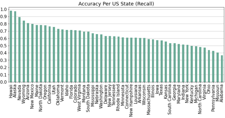
As before, we build a confusion matrix to examine patterns in the model’s errors, focusing on states with low accuracy such as Alabama, Michigan, and Pennsylvania:
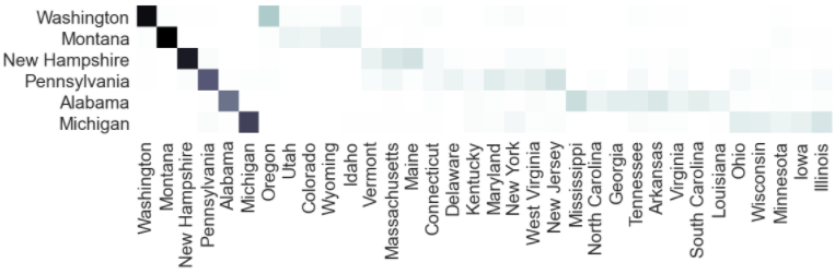
We observe that states are generally confused with other states in their geographic vicinity. For example, Alabama is confused with Mississippi, Tennessee, Arkansas, and Georgia, whereas New Hampshire is confused with Vermont, Massachusetts, Maine, and Connecticut.
As before, we examine precision and recall for each state. Keep in mind the following interpretations:
- State X has low recall: “Many locations in State X resemble other states”
- State Y has low precision: “Many locations in other states resemble State Y”
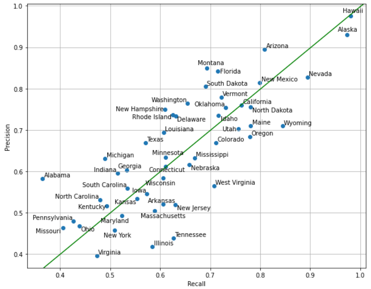
There are many states with lower recall than precision. Because all states are equally represented in the dataset, class imbalance cannot explain this (as it could in the case of the countries dataset). We examine the confusion matrix for precision. As before, each row contains all images predicted to be in State X, whereas the columns show where those images actually were.
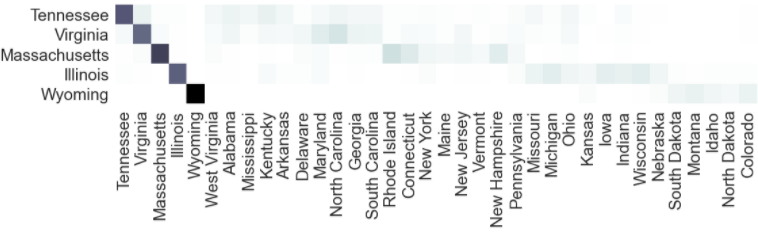
One intuitive explanation for a state having lower precision than recall is that it has become an archetype for a region. For example, we see that Massachusetts has become an archetype for the northeast, with images in states like New Hampshire and Rhode Island often getting classified as Massachusetts. Indeed, New Hampshire and Rhode Island both have much lower recall than precision, in part due to their images getting misclassified as Massachusetts. Similarly, Illinois is an archetype for the midwest, and Wyoming is an archetype for the rural west.
Location Prediction
We now have good classifiers for countries and US states, but we would also like to predict the precise location of an image. As a naive baseline, we can predict an image’s country, and use that country’s center as our location prediction. We compute a country’s center by taking the median latitude and longitude across all locations for that country in our training set. Following the convention of 2, 3, and 6, we report the fraction of test set images successfully localized within 1km (street), 25km (city), 200km (region), 750km (country), and 2500km (continent):
| Radius | Fraction of Images Successfully Localized Within Given Radius |
|---|---|
| 1km (0.6mi) | 0.07% |
| 25km (16mi) | 2.5% |
| 200km (124mi) | 18.7% |
| 750km (466mi) | 53.1% |
| 2500km (1553mi) | 83.4% |
This is a good start, but we would like to do better. Some countries like the US are so large that predicting the center is not a good approach. Intuitively, we should get better results by subdividing the world into pieces that are smaller than countries, and using the center of those small pieces as our predictions. The authors of PlaNet 2 do exactly this, and refer to these small pieces as “geocells.” The authors divided the world map into 26,263 geocells, each containing about 2,500 to 10,000 images. Unfortunately, our dataset is much smaller than theirs (97k vs 137m), so we must use a smaller number of larger geocells in order to have a sufficient number of training examples for each geocell.
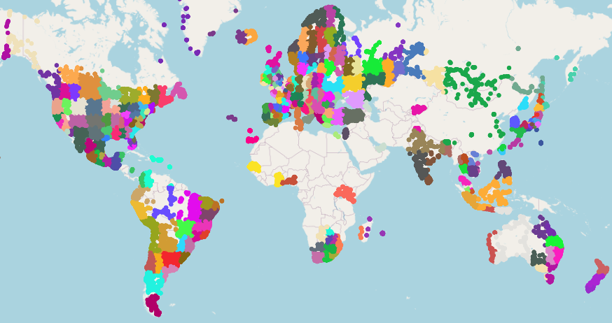
To create the geocells, we start by defining the world as one big geocell. Then, we recursively split geocells in half while they contain at least 600 images. The splits are somewhat random, but they favor splitting along the longer edge, as well as ensuring that the two resulting geocells contain a similar number of examples. Finally, we discard geocells with less than 50 examples. The result is 275 geocells containing an average of 353 examples each:
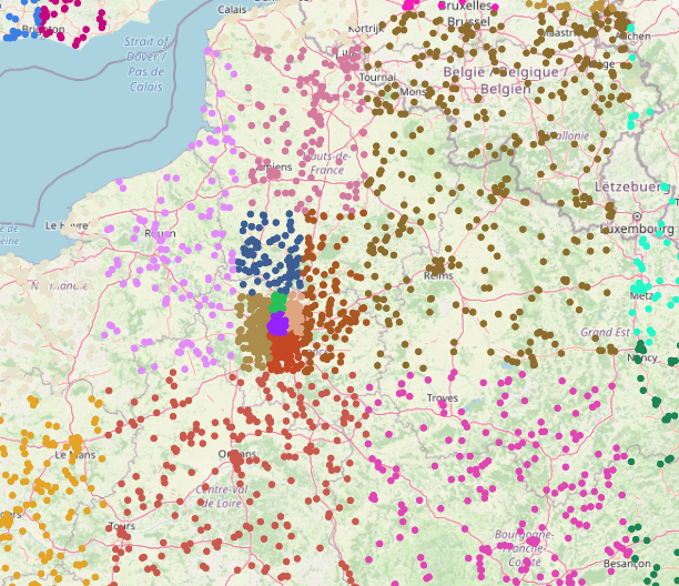
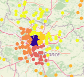
As expected, geocells are smaller in more densely populated areas. For example, there is one big green geocell that covers most of Mongolia, whereas there is a much higher density of geocells in Europe. As an extreme example, we examine the geocells in the vicinity of Paris, observing that the metropolitan area alone contains six geocells:
As before, we fine-tune a resnet101 for the geocell prediction task. The geocell prediction accuracy is as follows:
| Top-1 | Top-3 | Top-5 | |
|---|---|---|---|
| Accuracy | 34.8% | 59.5% | 71.1% |
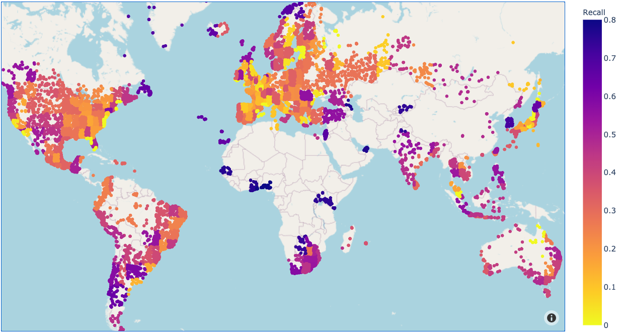
We can visualize the accuracy for each geocell, showing us which regions the model found it easier to classify. See the appendix for further error analysis.
We can now predict an image’s location by predicting its geocell, and using the geocell center as our guess. Like before, we compute the geocell center as the median latitude and longitude across all locations in our training set for that geocell. The results are as follows, including a comparison to our baseline country-center approach:
| Method | 1km (0.6mi) | 25km (16mi) | 200km (124mi) | 750km (466mi) | 2500km (1553mi) |
|---|---|---|---|---|---|
| Country Center | 0.07% | 2.5% | 18.7% | 53.1% | 83.4% |
| Geocell Center | 0.10% | 4.7% | 31.0% | 67.3% | 85.5% |
This is a clear improvement, especially for the 25-250km ranges. However, we’d still like to do better. We do so by using a KNN as in Vo et al 6. To compute the vector representation of an image, we run it through each of our three models (country, geocell, US state), and concanente the output logits into a length-412 vector (87 countries + 275 geocells + 50 states). We can then perform KNN using these vectors. We compute the similarity score between two vectors as follows. Increasing M will increase the model’s preference for the closest neighbors.
\[d(v_1, v_2) = \frac{1}{ ( || v_1 - v_2 ||_2 ) ^M}\]After finding the K closest neighbors for a given image, we need to take some sort of weighted average of these K neighbors to predict a single location. As described in Vo et al 6, we do so by plotting a gaussian filter (essentially a 2D bell curve) at each of the K locations. We scale each gaussian filter by that location’s similarity score, as defined above. The point with the highest density is our final prediction. Consider this example:
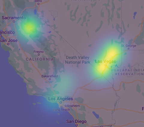
In this hypothetical scenario, we set K=5 and observe that one of the nearest neighbors is near Sacramento, two are near Las Vegas, and two are near Los Angeles. The locations in Sacramento and Las Vegas all have a high similarity score, whereas the two locations in Los Angeles have a lower similarity score, as indicated by the lesser intensity of those gaussian filters. The point with highest density (visually, the brightest point) turns out to be at the intersection of the two gaussian filters in Las Vegas. Therefore, this would be our predicted location.
In addition to K and M, we must also choose the hyperparameter σ, corresponding to the standard deviation for each gaussian filter. We experimentally chose the values K=20, M=2, and σ=4.
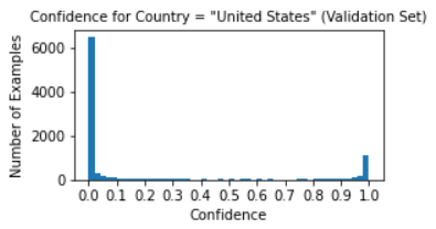
Note that there are three sets of features we are using to compute similarity: country logits, geocell logits, and US state logits. Does it make sense to weigh them all equally? Should we have different weightings for images that are in the US versus images that are not? To find out, we first divide our images into two groups: those that are in the US, and those that are not. In order for this operation to be reproducible on unlabeled images, we use our country-prediction model’s output to decide if a given image is in the US, using a threshold of 90% (eg. we say an image is in the US when our model is at least 90% confident of this). We chose this threshold based off our model’s confidence distribution:
We experimentally found that the optimal KNN feature weightings were as follows (we tested in increments of 0.1):
| Country Logits | Geocell Logits | State Logits | |
|---|---|---|---|
| US Images | 1.0 | 0.9 | 1.1 |
| Non-US Images | 1.0 | 1.0 | 0.0 |
Our most important finding here was that we should not use the US state features in our KNN when predicting the location of images that are not in the US (observe that the corresponding weight was 0.0). Using these feature weightings, our KNN results on the test set are as follows (in comparison to our earlier methods):
| Method | 1km (0.6mi) | 25km (16mi) | 200km (124mi) | 750km (466mi) | 2500km (1553mi) |
|---|---|---|---|---|---|
| Country Center | 0.07% | 2.5% | 18.7% | 53.1% | 83.4% |
| Geocell Center | 0.10% | 4.7% | 31.0% | 67.3% | 85.5% |
| KNN (σ=0) | 2.1% | 8.3% | 27.8% | 63.7% | 85.1% |
| KNN (σ=1) | 0.59% | 9.4% | 35.8% | 69.2% | 87.1% |
| KNN (σ=2) | 0.32% | 6.39% | 38.7% | 70.8% | 87.4% |
| KNN (σ=4) | 0.12% | 4.06% | 37.3% | 72.1% | 87.5% |
The KNN method is a clear improvement. We also included results for varying σ: a smaller value corresponds to tighter gaussian filters, and thus a stronger preference for the closest neighbors. In the extreme, σ=0 corresponds to 1 Nearest-Neighbor. Observe the tradeoff between accuracies at different thresholds as we vary σ. At σ=0 the accuracy within 1km is an impressive 2.1%, while the accuracy for higher thresholds is relatively low (being outperformed by our baseline methods). As we increase σ, the accuracy at higher thresholds increases, whereas the accuracy at lower thresholds decreases. Intuitively, this is because with a large value of σ, the model will choose a “safer” prediction that represents an average among likely locations, but is unlikely to be very close to the correct one. For our final model, we choose σ=2 as a good compromise.
So why did the KNN approach work? Vo et al 6 hypothesize that while neural networks are good at capturing features of an image, they are not as good at memorizing locations, since there are simply too many locations in the world for it to learn. They argue that KNN remains the best approach for geolocating images, as it can simply find the most similar images in its database. In other words, a neural network excels at feature extraction, while a KNN excels at instance matching. In our case, the features extracted by our country-prediction, geocell-prediction, and US state-prediction models correspond to how much a given image resembles each country, geocell, and US state, respectively. One could potentially improve on our result by training more nets to extract additional features.
Countries That Resemble US States
Just for fun, we apply our US state-classification model to images from other countries. Because the state-classification model was only trained on the dataset from Suresh et al 5, we can safely examine its output for all images in the dataset we scraped. We do this as follows: for a given Country X, we take the average prediction of our state-classification model across all images from Country X. The result is a length-50 vector that sums to one showing how much Country X looks like each of the 50 US States. For a given state, we can now find which countries resemble it the most:
| Country | Resemblance to Alaska |
|---|---|
| Finland | 38.7% |
| Norway | 29.2% |
| Sweden | 16.1% |
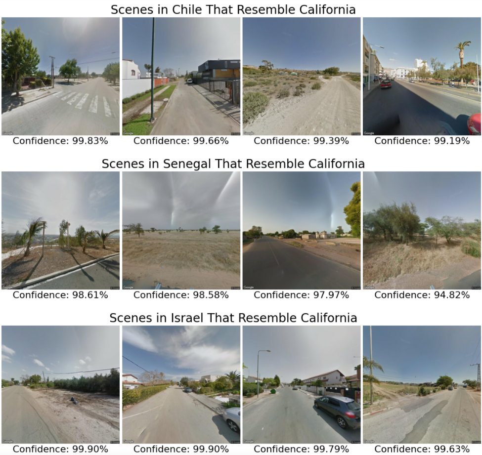
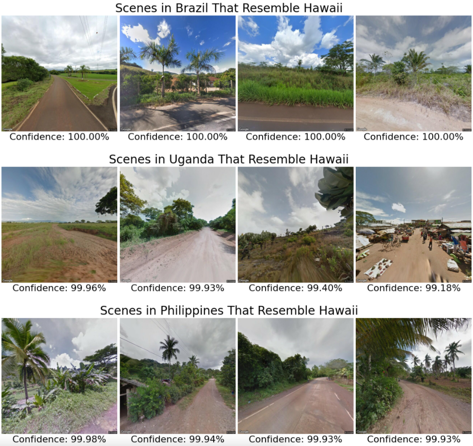
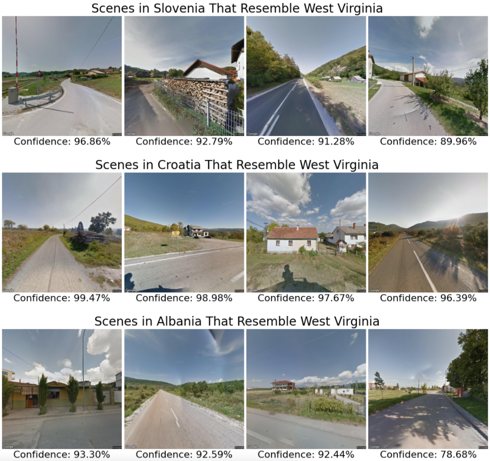
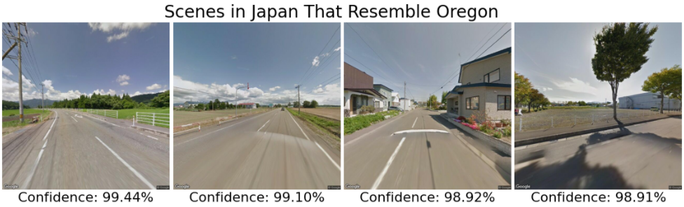
We can interpret this result as follows: “for an average image in Finland, our state-classification model is 38.7% confident that it is located in Alaska.” Similar interpretations apply for Norway and Sweden. Let’s look at the four images from Finland (resp. Norway) that our model was most confident were located in Alaska (the confidence is reported below each image):
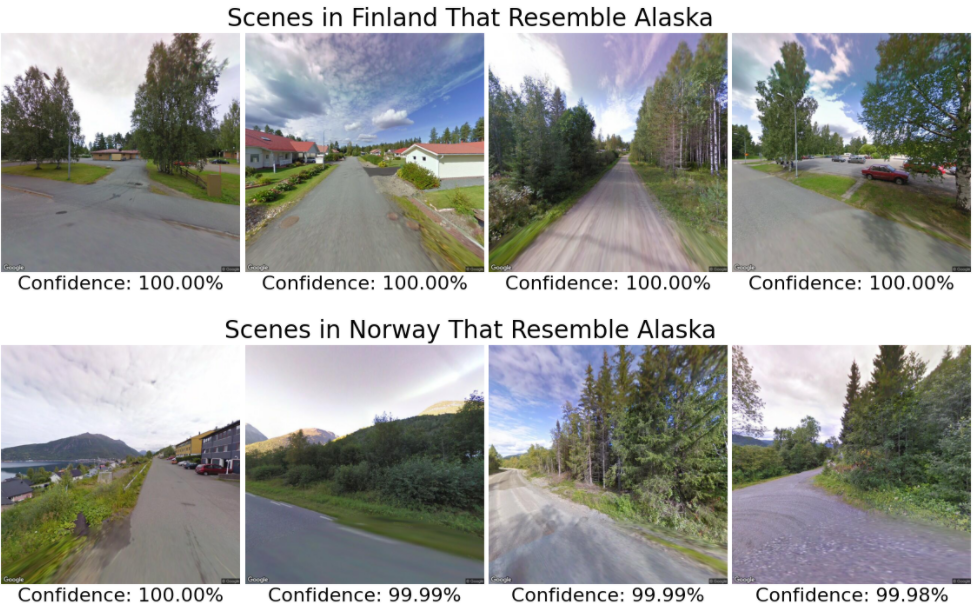
Indeed, these scenes do look similar to Alaska: they contain mountains, tall pine trees, and generally feel like they come from a northern climate. We do a similar analysis for Pennsylvania:
| Country | Resemblance to Pennsylvania |
|---|---|
| Czech Republic | 26.1% |
| Poland | 25.0% |
| Slovakia | 24.0% |
| Austria | 22.3% |
| Serbia | 22.2% |
| Germany | 22.0% |
| Hungary | 21.6% |
| Belgium | 21.5% |
| Macedonia | 21.3% |
| Netherlands | 21.2% |
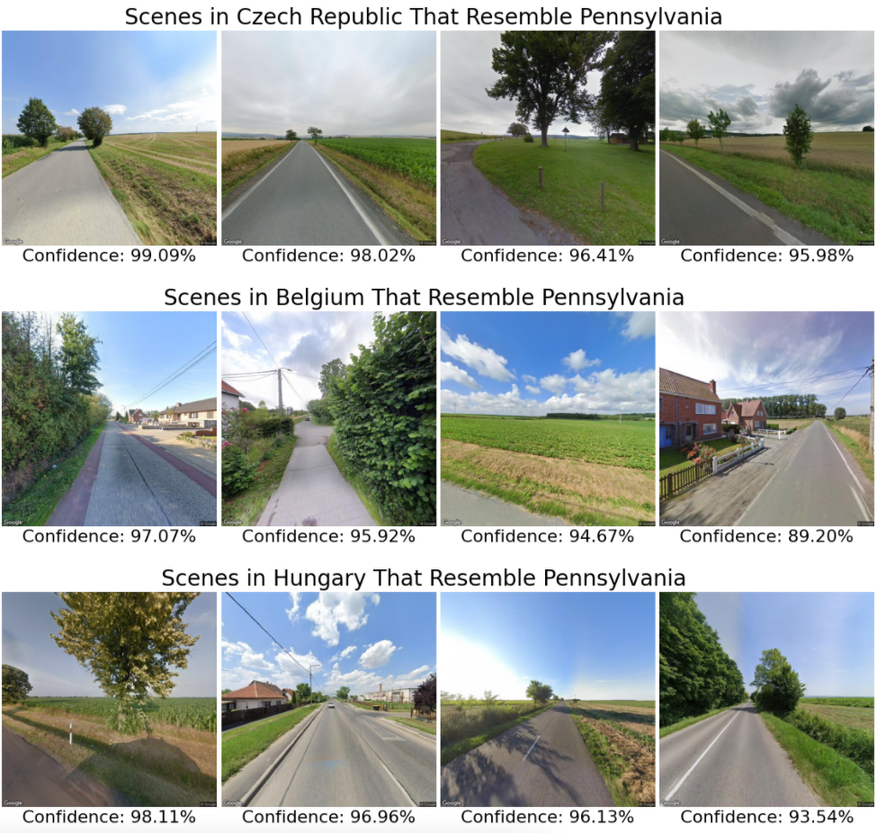
This time, it looks like the model is focusing on flat green fields with scattered trees. We present results from a few more states for the reader’s enjoyment:
| Country | Resemblance to California |
|---|---|
| Tunisia | 42.1% |
| Israel | 38.0% |
| Jordan | 26.6% |
| Senegal | 22.9% |
| Chile | 21.3% |
| Kyrgyzstan | 20.2% |
| Australia | 19.1% |
| United Arab Emirates | 18.6% |
| Spain | 18.0% |
| Greece | 17.9% |
| Country | Resemblance to Hawaii |
|---|---|
| American Samoa | 53.0% |
| Uganda | 47.4% |
| South Africa | 36.1% |
| Sri Lanka | 28.2% |
| Brazil | 28.1% |
| Philippines | 25.9% |
| Cambodia | 25.7% |
| Portugal | 24.0% |
| Ireland | 22.5% |
| Indonesia | 22.3% |
| Country | Resemblance to West Virginia |
|---|---|
| Bhutan | 32.3% |
| Slovenia | 28.8% |
| Croatia | 23.7% |
| Albania | 23.0% |
| Serbia | 20.7% |
| Faroe Islands | 20.2% |
| Macedonia | 19.9% |
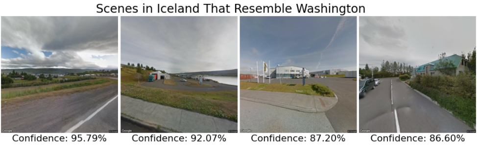
| Country | Resemblance to Oregon |
|---|---|
| Iceland | 20.7% |
| Japan | 14.4% |
| United Kingdom | 13.2% |
| Switzerland | 13.2% |
| New Zealand | 13.1% |
| Country | Resemblance to Oregon |
|---|---|
| Iceland | 23.2% |
| Greenland | 18.4% |
| Germany | 14.0% |
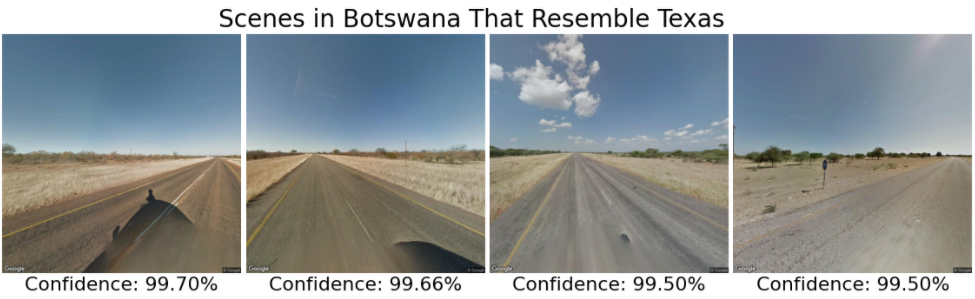
| Country | Resemblance to Texas |
|---|---|
| Botswana | 28.1% |
Appendix
Distribution of Dataset Across Countries
The team at GeoGuessr provided us with a list of 100,000 locations, from which we created a dataset of 97,068 locations and images. To assess how uniformly these locations are distributed around the world, we examine the relationship between a country’s population and the number of images from that country in our dataset:
| Country | Population (millions) | Dataset Count | Pop per Datum (thousands) |
|---|---|---|---|
| United States | 323.13 | 19007 | 17.0 |
| France | 66.90 | 6117 | 10.9 |
| Russia | 144.34 | 5399 | 26.7 |
| Japan | 126.99 | 5161 | 24.6 |
| United Kingdom | 65.64 | 4825 | 13.6 |
| Brazil | 207.65 | 4442 | 46.7 |
| Canada | 36.29 | 3624 | 10.0 |
| Mexico | 127.54 | 3480 | 36.6 |
| Spain | 46.44 | 3267 | 14.2 |
| Australia | 24.13 | 3246 | 7.4 |
| South Africa | 55.91 | 2437 | 22.9 |
| Italy | 60.60 | 1947 | 31.1 |
| Norway | 5.23 | 1897 | 2.8 |
| Poland | 37.95 | 1732 | 21.9 |
| Finland | 5.50 | 1723 | 3.2 |
| Sweden | 9.90 | 1640 | 6.0 |
| Argentina | 43.85 | 1538 | 28.5 |
| Thailand | 68.86 | 1371 | 50.2 |
| Romania | 19.71 | 1163 | 16.9 |
| New Zealand | 4.69 | 1139 | 4.1 |
The “Pop Per Datum” column is a ratio computed as (Country X population) / (number of dataset entries in Country X) * 1000. A low number means that the country is overrepresented in the dataset, whereas a high number means that it is underrepresented. In general, this ratio is fairly consistent.
There is some imbalance, but it generally reflects the amount of Street View coverage that exists in a given country. For example, countries like Brazil which have sparse Street View coverage are underrepresented in our dataset, whereas countries like Finland with comprehensive Street View coverage are overrepresented. We chose not to implement class weightings to fix this imbalance for two reasons: first, the imbalance is representative of the actual distribution of images one would see while playing GeoGuessr, and second, because the imbalance is generally not too severe.
Geocell Classification Error Analysis
Recall that our geocell prediction accuracy is as follows:
| Top-1 | Top-3 | Top-5 | |
|---|---|---|---|
| Accuracy | 34.8% | 59.5% | 71.1% |
Some geocells have much higher accuracy, such as this one in Paris, which has 74.4% accuracy:
Other geocells have lower accuracy: many are even 0%. Let’s examine one of these 0%-accuracy geocells. The yellow region corresponds to the actual geocell, and the darker regions correspond to the predicted geocells (across the validation and test sets):
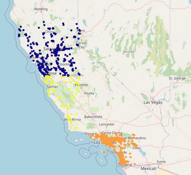
This geocell corresponds to central Californa. It is very small, only containing 28 elements across the validation and test sets. The model apparently decided to err in favor of the larger geocells encompassing San Francisco and Los Angeles. Let’s examine another 0%-accuracy geocell:
This geocell is also quite small, only containing 21 images in in the validation and test sets. As before, the model errs in favor of larger geocells. This geocell also straddles two countries separated by a large body of water. This not only makes it harder for the model to classify it correctly, but it also makes geolocation harder, as the two clusters in the geocell are quite far apart. A smarter geocell creation method may be able to mitigate both of the problems we’ve noted by creating equally-sized geocells (no small ones), and by not creating geocells that encompass different countries.
Footnotes
-
James Hays, Alexei A. Efros. IM2GPS: estimating geographic information from a single image. Proceedings of the IEEE Conf. on Computer Vision and Pattern Recognition (CVPR), 2008. ↩
-
Weyand, Tobias, et al. “PlaNet - Photo Geolocation with Convolutional Neural Networks.” ArXiv:1602.05314 [Cs], vol. 9912, 2016, pp. 37–55. arXiv.org, doi:10.1007/978-3-319-46484-8_3. ↩ ↩2 ↩3
-
Eric Muller-Budack, Kader Pustu-Iren, and Ralph Ewerth. 2018. Geolocation Estimation of Photos using a Hierarchical Model and Scene Classification. In Proceedings of the European Conference on Computer Vision. ↩ ↩2
-
A. R. Zamir and M. Shah. Accurate Image Localization Based on Google Maps Street View. In ECCV, 2010. ↩
-
Suresh, Sudharshan, et al. “DeepGeo: Photo Localization with Deep Neural Network.” ArXiv:1810.03077 [Cs], Oct. 2018. arXiv.org, http://arxiv.org/abs/1810.03077. ↩ ↩2 ↩3 ↩4
-
Vo, Nam, et al. “Revisiting IM2GPS in the Deep Learning Era.” ArXiv:1705.04838 [Cs], May 2017. arXiv.org, http://arxiv.org/abs/1705.04838. ↩ ↩2 ↩3 ↩4